QUANTIZING THE ELECTROMAGNETIC FIELD TO CALCULATE ELECTRONS - PHOTONS INTERACTIONS
The process of quantizing a scalar boson field is achieved with the classical field being decomposed into normal modes, and each mode is quantized by assigning it an independent set of creation and annihilation operators. By comparing the oscillator energies in the classical and quantum regimes, we can derive the Hermitian operator corresponding to the classical field variable, expressed using the creation and annihilation operators. The same approach will be used with some minor adjustments, to quantize the electromagnetic field.
First, consider a “source-free” electromagnetic field—i.e., with no electric charges and currents. Without sources, Maxwell’s equations (in SI units, and in a vacuum) reduce to:
\[\begin{align} \nabla\cdot \mathbf{E} &= 0 \label{max1} \\ \nabla\cdot \mathbf{B} &= 0 \label{max2}\\ \nabla\times \mathbf{E} &= -\frac{\partial \mathbf{B}}{\partial t} \label{max3}\\ \nabla\times \mathbf{B} &= \frac{1}{c^2} \frac{\partial \mathbf{E}}{\partial t}. \label{max4}\end{align}\]
Once again, we introduce the scalar potential \(\Phi\) and vector potential \(\mathbf{A}\):
\[\begin{align} \mathbf{E} &= - \nabla \Phi - \frac{\partial\mathbf{A}}{\partial t} \label{Efield} \\ \mathbf{B} &= \nabla \times \mathbf{A}. \label{Bfield}\end{align}\]
With these relations, Equations \(\eqref{max2}\) and \(\eqref{max3}\) are satisfied automatically via vector identities. The two remaining equations, \(\eqref{max1}\) and \(\eqref{max4}\), become:
\[\begin{align} \nabla^2 \Phi &= -\frac{\partial}{\partial t} \nabla \cdot \mathbf{A} \label{max5} \\ \left(\nabla^2 - \frac{1}{c^2}\frac{\partial^2}{\partial t^2}\right) \mathbf{A} &= \nabla\left[\frac{1}{c^2}\frac{\partial}{\partial t} \Phi + \nabla\cdot\mathbf{A}\right]. \label{max6}\end{align}\]
In the next step, we choose a convenient gauge called the Coulomb gauge:
\[\Phi = 0, \;\;\; \nabla \cdot \mathbf{A} = 0. \label{coulomb}\]
(To see that we can always make such a gauge choice, suppose we start out with a scalar potential \(\Phi_0\) and vector potential \(\mathbf{A}_0\) not satisfying \(\eqref{coulomb}\). Perform a gauge transformation with a gauge field \(\Lambda(\mathbf{r}, t) = - \int^t dt'\; \Phi_0(\mathbf{r}, t')\). The new scalar potential is \(\Phi = \Phi_0 + \dot{\Lambda} = 0\); moreover, the new vector potential satisfies
\[\nabla\cdot\mathbf{A} = \nabla\cdot \mathbf{A}_0 - \nabla^2 \Lambda = \nabla\cdot \mathbf{A}_0 + \int^t dt'\; \nabla^2\Phi_0(\mathbf{r}, t').\]
Upon using Equation \(\eqref{max5}\), we find that \(\nabla\cdot\mathbf{A} = 0\).)
In the Coulomb gauge, Equation \(\eqref{max5}\) is automatically satisfied. The sole remaining equation, \(\eqref{max6}\), simplifies to
\[\left(\nabla^2 - \frac{1}{c^2}\frac{\partial^2}{\partial t^2}\right) \mathbf{A} = 0. \label{max8}\]
This has plane-wave solutions of the form
\[\mathbf{A}(\mathbf{r},t) = \Big(\mathcal{A}\, \, e^{i(\mathbf{k}\cdot\mathbf{r} - \omega t)} + \mathrm{c.c.}\Big)\, \mathbf{e}, \label{lightplanewave}\]
where \(\mathcal{A}\) is a complex number (the mode amplitude) that specifies the magnitude and phase of the plane wave, \(\mathbf{e}\) is a real unit vector (the polarization vector) that specifies which direction the vector potential points along, and “c.c.” denotes the complex conjugate of the first term. Referring to Equation \(\eqref{max8}\), the angular frequency \(\omega\) must satisfy
\[\omega = c|\mathbf{k}|.\]
Moreover, since \(\nabla \cdot \mathbf{A} = 0\), it must be the case that
\[\mathbf{k} \cdot \mathbf{e} = 0.\]
In other words, the polarization vector is perpendicular to the propagation direction. For any given \(\mathbf{k}\), we can choose (arbitrarily) two orthogonal polarization vectors.
Now suppose we put the electromagnetic field in a box of volume \(V = L^3\), with periodic boundary conditions (we will take \(L \rightarrow \infty\) at the end). The \(\mathbf{k}\) vectors form a discrete set:
\[k_j = \frac{2\pi n_j}{L}, \;\; n_j \in \mathbf{Z}, \;\;\mathrm{for} \;\; j = 1,2,3.\]
Then the vector potential field can be decomposed as a superposition of plane waves,
\[\mathbf{A}(\mathbf{r},t) = \sum_{\mathbf{k}\lambda} \Big(\mathcal{A}_{\mathbf{k}\lambda} \, e^{i(\mathbf{k}\cdot\mathbf{r} - \omega_{\mathbf{k}} t)} + \mathrm{c.c.}\Big)\, \mathbf{e}_{\mathbf{k}\lambda}, \;\;\; \mathrm{where} \;\;\;\omega_{\mathbf{k}} = c|\mathbf{k}|.\]
Here, \(\lambda\) is a two-fold polarization degree of freedom indexing the two possible orthogonal polarization vectors for each \(\mathbf{k}\). (We won’t need to specify how exactly these polarization vectors are defined, so long as the definition is used consistently.)
To convert the classical field theory into a quantum field theory, for each \((\mathbf{k},\lambda)\) we define an independent set of creation and annihilation operators:
\[\big[\hat{a}_{\mathbf{k}\lambda}, \hat{a}_{\mathbf{k}'\lambda'}^\dagger\big] = \delta_{\mathbf{k}\mathbf{k}'} \delta_{\lambda\lambda'}, \;\;\; \big[\hat{a}_{\mathbf{k}\lambda}, \hat{a}_{\mathbf{k}'\lambda'}\big] = \big[\hat{a}_{\mathbf{k}\lambda}^\dagger, \hat{a}_{\mathbf{k}'\lambda'}^\dagger\big] = 0.\]
Then the Hamiltonian for the electromagnetic field is
\[\hat{H} = \sum_{\mathbf{k}\lambda} \hbar \omega_{\mathbf{k}} \, \hat{a}^\dagger_{\mathbf{k}\lambda} \hat{a}_{\mathbf{k}\lambda}, \;\;\; \mathrm{where} \;\;\;\omega_{\mathbf{k}} = c|\mathbf{k}|.\]
The vector potential is now promoted into a Hermitian operator in the Heisenberg picture:
\[\hat{\mathbf{A}}(\mathbf{r},t) = \sum_{\mathbf{k}\lambda} \mathcal{C}_{\mathbf{k}\lambda}\, \Big(\hat{a}_{\mathbf{k}\lambda} \, e^{i(\mathbf{k}\cdot\mathbf{r} - \omega_{\mathbf{k}} t)} + \mathrm{h.c.}\Big)\, \mathbf{e}_{\mathbf{k}\lambda}. \label{Aquantum}\]
Here, \(\mathcal{C}_{\mathbf{k}\lambda}\) is a constant to be determined, and “h.c.” denotes the Hermitian conjugate. The creation and annihilation operators in this equation are Schrödinger picture (\(t = 0\)) operators. The particles they create/annihilate are photons—elementary particles of light.
To find \(\mathcal{C}_{\mathbf{k}\lambda}\), we compare the quantum and classical energies. Suppose the electromagnetic field is in a coherent state \(|\alpha\rangle\) such that for any \(\mathbf{k}\) and \(\lambda\),
\[\hat{a}_{\mathbf{k}\lambda}|\alpha\rangle = \alpha_{\mathbf{k}\lambda}|\alpha\rangle \label{coherent}\]
for some \(\alpha_{\mathbf{k}\lambda} \in \mathbb{C}\). From this and Equation \(\eqref{Aquantum}\), we identify the corresponding classical field
\[\mathbf{A}(\mathbf{r},t) = \sum_{\mathbf{k}\lambda} \Big(\mathcal{A}_{\mathbf{k}\lambda}\, e^{i(\mathbf{k}\cdot\mathbf{r} - \omega_{\mathbf{k}} t)} + \mathrm{c.c.}\Big)\, \mathbf{e}_{\mathbf{k}\lambda}, \quad \mathrm{where}\;\;\; \mathcal{C}_{\mathbf{k}\lambda} \alpha_{\mathbf{k}\lambda} = \mathcal{A}_{\mathbf{k}\lambda}.\]
For each \(\mathbf{k}\) and \(\lambda\), Equations \(\eqref{Efield}\)–\(\eqref{Bfield}\) give the electric and magnetic fields
\[\begin{align} \mathbf{E}_{\mathbf{k}\lambda} &= \Big(i\omega_{\mathbf{k}} \mathcal{A}_{\mathbf{k}\lambda}\, e^{i(\mathbf{k}\cdot\mathbf{r} - \omega_{\mathbf{k}} t)} + \mathrm{c.c.}\Big)\, \mathbf{e}_{\mathbf{k}\lambda} \\ \mathbf{B}_{\mathbf{k}\lambda} &= \Big(i \mathcal{A}_{\mathbf{k}\lambda}\, e^{i(\mathbf{k}\cdot\mathbf{r} - \omega_{\mathbf{k}} t)} + \mathrm{c.c.}\Big) \; \mathbf{k} \times \mathbf{e}_{\mathbf{k}\lambda}.\end{align}\]
In the classical theory of electromagnetism, Poynting’s theorem tells us that the total energy carried by a classical plane electromagnetic wave is
\[\begin{align} \begin{aligned} E &= \int_V d^3\!r\; \frac{\epsilon_0}{2} \left( \big|\mathbf{E}_{\mathbf{k}\lambda}\big|^2 + c^2 \big|\mathbf{B}_{\mathbf{k}\lambda}\big|^2 \right) \\ &= 2 \, \epsilon_0\, \omega_{\mathbf{k}}^2 \; |\mathcal{A}_{\mathbf{k}\lambda}|^2 \,V. \end{aligned}\end{align}\]
Here, \(V\) is the volume of the enclosing box, and we have used the fact that terms like \(e^{2i\mathbf{k}\cdot\mathbf{r}}\) vanish when integrated over \(\mathbf{r}\). Hence, we make the correspondence
\[2\,\epsilon_0\, \omega_{\mathbf{k}}^2 \, |\mathcal{C}_{\mathbf{k}\lambda}\alpha_{\mathbf{k}\lambda}|^2 \, V = \hbar \omega_{\mathbf{k}} |\alpha_{\mathbf{k}\lambda}|^2 \quad \Rightarrow\;\;\; \mathcal{C}_{\mathbf{k}\lambda} = \sqrt{\frac{\hbar}{2\epsilon_0\omega_{\mathbf{k}}V}}.\]
We thus arrive at the result
\[\begin{align} \begin{aligned} \hat{H} &= \sum_{\mathbf{k}\lambda} \hbar \omega_{\mathbf{k}} \, \hat{a}^\dagger_{\mathbf{k}\lambda} \hat{a}_{\mathbf{k}\lambda} \\ \hat{\mathbf{A}}(\mathbf{r},t) &= \sum_{\mathbf{k}\lambda} \sqrt{\frac{\hbar}{2\epsilon_0\omega_{\mathbf{k}}V}}\, \Big(\hat{a}_{\mathbf{k}\lambda} \, e^{i(\mathbf{k}\cdot\mathbf{r} - \omega_{\mathbf{k}} t)} + \mathrm{h.c.}\Big)\, \mathbf{e}_{\mathbf{k}\lambda} \\ \omega_{\mathbf{k}} &= c|\mathbf{k}|, \;\;\; \big[\hat{a}_{\mathbf{k}\lambda}, \hat{a}_{\mathbf{k}'\lambda'}^\dagger\big] = \delta_{\mathbf{k}\mathbf{k}'} \delta_{\lambda\lambda'}, \;\;\; \big[\hat{a}_{\mathbf{k}\lambda}, \hat{a}_{\mathbf{k}'\lambda'}\big] = 0. \end{aligned} \label{qed1} \end{align}\]
To describe infinite free space rather than a finite-volume box, we take the \(L\rightarrow \infty\) limit and re-normalize the creation and annihilation operators by the replacement
\[\hat{a}_{\mathbf{k}\lambda} \rightarrow \sqrt{\frac{(2\pi)^3}{V}} \; \hat{a}_{\mathbf{k}\lambda}.\]
Then the sums over \(\mathbf{k}\) become integrals over the infinite three-dimensional space:
\[\begin{align} \begin{aligned} \hat{H} &= \int d^3k\sum_{\lambda} \hbar \omega_{\mathbf{k}} \, \hat{a}^\dagger_{\mathbf{k}\lambda} \hat{a}_{\mathbf{k}\lambda} \\ \hat{\mathbf{A}}(\mathbf{r},t) &= \int d^3k \sum_{\lambda} \sqrt{\frac{\hbar}{16\pi^3\epsilon_0\omega_{\mathbf{k}}}}\, \Big(\hat{a}_{\mathbf{k}\lambda} \, e^{i(\mathbf{k}\cdot\mathbf{r} - \omega_{\mathbf{k}} t)} + \mathrm{h.c.}\Big)\, \mathbf{e}_{\mathbf{k}\lambda} \\ \omega_{\mathbf{k}} &= c|\mathbf{k}|, \;\;\; \big[\hat{a}_{\mathbf{k}\lambda}, \hat{a}_{\mathbf{k}'\lambda'}^\dagger\big] = \delta^3(\mathbf{k}-\mathbf{k}') \delta_{\lambda\lambda'}, \;\;\; \big[\hat{a}_{\mathbf{k}\lambda}, \hat{a}_{\mathbf{k}'\lambda'}\big] = 0. \end{aligned} \label{qed2}\end{align}\]
ELECTRON-PHOTON INTERACTION
Having derived quantum theories for the electron and the electromagnetic field, we can put them together to describe how electrons interact with the electromagnetic field by absorbing and/or emitting photons. Here, we present the simplest such calculation.
Let \(\mathscr{H}_{\mathrm{e}}\) be the Hilbert space for one electron, and \(\mathscr{H}_{\mathrm{EM}}\) be the Hilbert space for the electromagnetic field. The combined system is thus described by \(\mathscr{H}_e \otimes \mathscr{H}_{\mathrm{EM}}\). We seek a Hamiltonian of the form
\[H = H_e + H_{\mathrm{EM}} + H_{\mathrm{int}},\]
where \(H_e\) is the Hamiltonian for the “bare” electron, \(H_{\mathrm{EM}}\) is the Hamiltonian for the source-free electromagnetic field, and \(H_{\mathrm{int}}\) is an interaction Hamiltonian describing how the electron interacts with photons.
Let us once again adopt the Coulomb gauge, so that the scalar potential is zero, and the electromagnetic field is solely described via the vector potential. In Section 5.1, we saw that the effect of the vector potential on a charged particle can be described via the substitution
\[\hat{\mathbf{p}} \rightarrow \hat{\mathbf{p}} + e\mathbf{A}(\hat{\mathbf{r}},t).\]
In Section 5.2, we saw that this substitution is applicable not just to non-relativistic particles, but also to fully relativistic particles described by the Dirac Hamiltonian. Previously, we have treated the \(\mathbf{A}\) in this substitution as a classical object lacking quantum dynamics of its own. Now, we replace it by the vector potential operator derived in Section 5.3:
\[\hat{\mathbf{A}}(\hat{\mathbf{r}},t) = \begin{cases} \displaystyle \sum_{\mathbf{k}\lambda} \sqrt{\frac{\hbar}{2\epsilon_0\omega_{\mathbf{k}}V}}\, \Big(\hat{a}_{\mathbf{k}\lambda} \, e^{i(\mathbf{k}\cdot\mathbf{r} - \omega_{\mathbf{k}} t)} + \mathrm{h.c.}\Big)\, \mathbf{e}_{\mathbf{k}\lambda}, & (\mathrm{finite}\;\mathrm{volume}) \\ \displaystyle \int d^3k \sum_{\lambda} \sqrt{\frac{\hbar}{16\pi^3\epsilon_0\omega_{\mathbf{k}}}}\, \Big(\hat{a}_{\mathbf{k}\lambda} \, e^{i(\mathbf{k}\cdot\hat{\mathbf{r}} - \omega_{\mathbf{k}} t)} + \mathrm{h.c.}\Big)\, \mathbf{e}_{\mathbf{k}\lambda}, & (\mathrm{infinite}\;\mathrm{space}). \end{cases} \label{Aoperator}\]
Using this, together with either the electronic and electromagnetic Hamiltonians, we can finally describe the photon emission process. Suppose a non-relativistic electron is orbiting an atomic nucleus in an excited state \(|1\rangle \in \mathscr{H}_e\). Initially, the photon field is in its vacuum state \(|\varnothing\rangle \in \mathscr{H}_{\mathrm{EM}}\). Hence, the initial state of the combined system is
\[|\psi_i\rangle = |1\rangle \otimes |\varnothing\rangle.\]
Let \(H_{\mathrm{int}}\) be the Hamiltonian term responsible for photon absorption/emission. If \(H_{\mathrm{int}} = 0\), then \(|\psi_i\rangle\) would be an energy eigenstate. The atom would remain in its excited state forever.
In actuality, \(H_{\mathrm{int}}\) is not zero, so \(|\psi_i\rangle\) is not an energy eigenstate. As the system evolves, the excited electron may decay into its ground state \(|0\rangle\) by emitting a photon with energy \(E\), equal to the energy difference between the atom’s excited state \(|1\rangle\) and ground state \(|0\rangle\). For a non-relativistic electron, the Hamiltonian (5.1.20) yields the interaction Hamiltonian
\[H_{\mathrm{int}} = \frac{e}{2m} \left( \hat{\mathbf{p}} \cdot \hat{\mathbf{A}} + \mathrm{h.c.}\right),\]
where \(\hat{\mathbf{A}}\) must now be treated as a field operator, not a classical field.
Consider the states that \(|\psi_i\rangle\) can decay into. There is a continuum of possible final states, each having the form
\[| \psi_{f}^{(\mathbf{k}\lambda)} \rangle = |0\rangle \otimes \left( \hat{a}_{\mathbf{k}\lambda}^\dagger |\varnothing\rangle\right), \label{decaystate}\]
which describes the electron being in its ground state and the electromagnetic field containing one photon, with wave-vector \(\mathbf{k}\) and polarization \(\lambda\).
According to Fermi’s Golden Rule, the decay rate is
\[\kappa = \frac{2\pi}{\hbar} \; \overline{\Big| \langle \psi_{f}^{(\mathbf{k}\lambda)} | \hat{H}_{\mathrm{int}}|\psi_i\rangle\Big|^2} \; \mathcal{D}(E),\]
where \(\overline{(\cdots)}\) denotes the average over the possible decay states of energy \(E\) (i.e., equal to the energy of the initial state), and \(\mathcal{D}(E)\) is the density of states.
To calculate the matrix element \(\langle \psi_{f}^{(\mathbf{k}\lambda)}| \hat{H}_{\mathrm{int}}|\psi_i\rangle\), let us use the infinite-volume version of the vector field operator \(\eqref{Aoperator}\). (You can check that using the finite-volume version yields the same results; see Exercise 5.5.2.) We will use the Schrödinger picture operator, equivalent to setting \(t = 0\) in Equation \(\eqref{Aoperator}\). Then
\[\begin{align} \begin{aligned} \langle \psi_{f}^{(\mathbf{k}\lambda)}| \hat{H}_{\mathrm{int}}|\psi_i\rangle &= \frac{e}{2m} \int d^3 k' \sum_{j\lambda} \sqrt{\frac{\hbar}{16\pi^3\epsilon_0 \omega_{\mathbf{k}'}}} \\ &\qquad\quad\times \Big( \langle 0 |\hat{p}_j e^{-i\mathbf{k}\cdot\hat{\mathbf{r}}} | 1 \rangle + \left\langle 0 |e^{-i\mathbf{k}\cdot\hat{\mathbf{r}}} \hat{p}_j| 1 \right\rangle \Big) \; e_{\mathbf{k}'\lambda'}^j \; \langle\varnothing|\hat{a}_{\mathbf{k}\lambda} \hat{a}_{\mathbf{k}'\lambda'}^\dagger|\varnothing\rangle. \end{aligned}\end{align}\]
We can now use the fact that \(\langle\varnothing|\hat{a}_{\mathbf{k}\lambda} \hat{a}_{\mathbf{k}'\lambda'}^\dagger|\varnothing\rangle = \delta^3(\mathbf{k}-\mathbf{k}') \delta_{\lambda\lambda'}\). Moreover, we approximate the \(\exp(-i\mathbf{k}\cdot\hat{\mathbf{r}})\) factors in the brakets with 1; this is a good approximation since the size of a typical atomic orbital (\(\lesssim 10^{-9}\,\textrm{m}\)) is much smaller than the optical wavelength (\(\sim 10^{-6}\,\textrm{m}\)), meaning that \(\exp(-i\mathbf{k}\cdot\mathbf{r})\) does not vary appreciably over the range of positions \(\mathbf{r}\) where the orbital wavefunctions are significant. The above equation then simplifies to
\[\langle \psi_{f}^{(\mathbf{k}\lambda)}| \hat{H}_{\mathrm{int}}|\psi_i\rangle \approx \frac{e}{m} \sum_{j} \sqrt{\frac{\hbar}{16\pi^3\epsilon_0 \omega_{\mathbf{k}}}} \;\; \langle 0 |\hat{p}_j|1 \rangle \; e_{\mathbf{k}\lambda}^j.\]
We can make a further simplification by observing that for \(\hat{H}_e = |\hat{\mathbf{p}}|^2/2m + V(\mathbf{r})\),
\[ [\hat{H}_{e},\: \hat{\mathbf{r}}]= -i\hbar\mathbf{p}/m \;\;\;\Rightarrow \;\;\; \langle 0|\hat{p}_j|1\rangle = - \frac{imE \mathbf{d}}{\hbar}.\]
The complex number \(\mathbf{d} = \langle 0 |\mathbf{r} | 1\rangle\), called the transition dipole moment, is easily calculated from the orbital wavefunctions. Thus,
\[\begin{align} \langle \psi_{f}^{(\mathbf{k}\lambda)}| \hat{H}_{\mathrm{int}}|\psi_i\rangle &\approx - ie \sqrt{\frac{E}{16\pi^3\epsilon_0}}\; \mathbf{d}\cdot \mathbf{e}_{\mathbf{k}\lambda}. \\ \big| \langle \psi_{f}^{(\mathbf{k}\lambda)}| \hat{H}_{\mathrm{int}} |\psi_i\rangle\big|^2 &\approx \frac{e^2E}{16\pi^3\epsilon_0}\; \big|\mathbf{d}\cdot \mathbf{e}_{\mathbf{k}\lambda}\big|^2. \label{transsq}\end{align}\]
(Check for yourself that Equation \(\eqref{transsq}\) should, and does, have units of \([E^2V]\).) We now need the average over the possible photon states (\(\mathbf{k}, \lambda\)). In taking this average, the polarization vector runs over all possible directions, and a standard angular integration shows that
\[\overline{|\mathbf{d}\cdot \mathbf{e}_{\mathbf{k}\lambda}|^2} \,=\, \sum_{j=1}^3 |d_j|^2 \;\overline{e_j^2} \,=\, \sum_{j=1}^3 |d_j|^2 \cdot \frac{1}{3} \,=\, \frac{|\mathbf{d}|^2}{3}.\]
\[\alpha = \frac{e^2}{4\pi\epsilon_0\hbar c} \approx \frac{1}{137}, \label{alpha}\]
and defining \(\omega = E / \hbar\) as the frequency of the emitted photon. The resulting decay rate is
Definition: Decay Rate
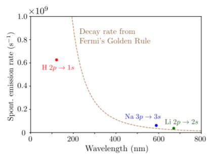
\[\kappa = \frac{4 \alpha \omega^3\, \overline{|\mathbf{d}|^2}}{3c^2}.\]
The image below compares this prediction to experimentally-determined decay rates for the simplest excited states of hydrogen, lithium, and sodium atoms. The experimental data are derived from atomic emission line-widths, and correspond to the rate of spontaneous emission (also called the “Einstein \(A\) coefficient”) as the excited state decays to the ground state. For the Fermi’s Golden Rule curve, we simply approximated the transition dipole moment as \(|\mathbf{d}| \approx 10^{-10}\,\mathrm{m}\) (based on the fact that \(|\mathbf{d}|\) has units of length, and the length scale of an atomic orbital is about an angstrom); to be more precise, \(\mathbf{d}\) ought to be calculated using the actual orbital wavefunctions. Even with the crude approximations we have made, the predictions are within striking distance of the experimental values.